What does all this mean? Let's talk about the components of the formula, and then apply it to an example: the website example of the probability that 2 (and only 2) skiers out of 5, each going down the hill one time, will break a leg.
Lecture 7 focuses on probability. There's some review here, but a lot
of this material is new.
As you may recall, aleatory just means 'pertaining to luck'.
But an aleatory probability generally means one that you can
calculate because you have perfect information about the system.
0 <= Pr(E) <= 1
In other words, the probability of any event is less than or equal to 1--
but greater than or equal to 0.
How would we express probability in general?
We would write:
PR (E) = number of ways in which E can occur
number of ways in which all equally likely events can occur (including E)
That is, the probability that an "event" (E) might occur can be calculated as
the number of ways in which the event can occur--divided by the total number of ways
in which all such events can occur.
The example that we used in lecture 6 was of a six sided fair die. So, answer
the following questions:
Pr (A or B) = Pr (A) + Pr (B)
Note that independent means that the two probabilities do not influence each other--the likelihood that one will happen does not influence the likelihood that the other will happen.
Given this,
Pr (A, B) = Pr(A) * Pr(B) . . . for independent events
That is, the probability of A and then B is equal to the probability of A multiplied by the probability of B.
Note that independent means that the two probabilities do not
influence each other--the likelihood that one will happen does not influence
the likelihood that the other will happen. The outcome of the first throw
does not influence the outcome of the second throw. In real life, beyond
throwing dice, outcomes are often not independent.
Given this,
Let's think about independence a bit more thoroughly.
Imagine one roll of a die--and consider two possible events.
Pr (A, B) = Pr (A) * Pr (B | A)
We say this: "The probability of A and then B is equal to the probability of A
plus the probability of B given A."
Essentially, what we're doing is breaking down the probabilities into independent probabilities. We
don't really want to add the probability of B to the probability of A--because we're only interested
in the probability of B if A happens.
_______________________________________
A couple of other notes:
1. P (B | A) = P (A and B) / P (A)
and so,
P (A or B) = P(A) + P(B) - P(A and B)
Note that this works for events that are mutually exclusive as well---because P(A and B)=0.Click
here to look at one of many websites available giving an overview of
binomial probability.
A few things that are relevant about binomial probabilities:
The formula for binomial probabilities is:

What does all this mean? Let's talk about the components of the formula,
and then apply it to an example: the website example of the probability
that 2 (and only 2) skiers out of 5, each going down the hill
one time, will break a leg.
Note that the first part of the right hand size--n! divided by
[x! (n-x)!]--is called the combinations formula. It tells you how
many combinations / ways there are in which the event you are interested in can
happen.
Let's think about the ski slope example. How can the combinations formula tell us
in how many combinations of trials two and only two skiers will break a leg?
So, what is N! in the ski slope example? Click
here for the answer.
What is the numerator for the above formula?
Click here
for the right answer.
What is the denominator for the above formula?
Click here for the answer.
So, what is the # of possible combinations--where two skiers out of
five total could (in any order) break their leg?
Click
here for the correct answer.
We can also think of this in terms of a tree diagram, where we can
outline all the possible combinations. NB stands for "not broken"--
"B" stands for broken. Each line below represents a possible
combination of the five skiers. Skier one is represented by
the first letter--he can either break his leg or not break his leg. So,
the first 16 cases represent the 16 possible combinations if skier
one breaks his leg. The second 16 cases represent the 16 possible combinations
if skier one doesn't break his leg. What happens to skier 2? Well, the
first eight cases represent the possible combinations if skier 2 breaks his leg--
given that skier 1 broke his leg. The second eight cases represent the
possible combinations if skier 2 doesn't break his leg--given that
skier 1 broke his leg. The third eight cases represent the possible
combinations if skier 2 breaks his leg--given that skier 1 didn't
break his leg. And the last (fourth) eight cases represent the possible
combinations if skier 2 doesn't break his leg -- given that skier 1 didn't break
his leg.
B --> B ----> B --->B---->B
B --> B ----> B --->B---->NB
B --> B ----> B --->NB--->B
B --> B ----> B --->NB--->NB
B --> B ----> NB--->B---->B
B --> B ----> NB--->B---->NB
B --> B ----> NB--->NB--->B
B --> B ----> NB--->NB--->NB

B --> NB ----> B --->B---->B
B --> NB ----> B --->B---->NB
B --> NB ----> B --->NB--->B
B --> NB ----> B --->NB--->NB
B --> NB ----> NB--->B---->B
B --> NB ----> NB--->B---->NB
B --> NB ----> NB--->NB--->B
B --> NB ----> NB--->NB--->NB

NB --> B ----> B --->B---->B
NB --> B ----> B --->B---->NB
NB --> B ----> B --->NB--->B
NB --> B ----> B --->NB--->NB
NB --> B ----> NB--->B---->B
NB --> B ----> NB--->B---->NB
NB --> B ----> NB--->NB--->B
NB --> B ----> NB--->NB--->NB

NB --> NB ----> B --->B---->B
NB --> NB ----> B --->B---->NB
NB --> NB ----> B --->NB--->B
NB --> NB ----> B --->NB--->NB
NB --> NB ----> NB--->B---->B
NB --> NB ----> NB--->B---->NB
NB --> NB ----> NB--->NB--->B
NB --> NB ----> NB--->NB--->NB
Count up how many combinations have two (and only two) skiers with
broken legs? What is the answer? And why? Click
here for the correct
answer.
As an aside, note that a general formula for the total combinations of outcomes is # possible individual outcomes to the power of # trials--in this case, 2 to the power of 5. 2 because there are always 2 possible outcomes, and then "the power of 5" because there are 5 skiers going down the hill; that is, five trials.
What is p, in this example of skiing? We know that p=.2. So, we can plug in p in the following way to the rest of the formula:
So, after plugging everything in, our new formula for this skiing case
looks like:

Which brings us to....

Which finally brings us to....

Let's think of a slightly more straightforward example. What is the probability of getting one and only one head if you toss a fair coin three times?
Note: you can also get the answer using the formula listed above
for total number of equally likely combinations; two (because for
each trial there are two possible outcomes: heads or tails) to the power
of three (because there are three trials) = 8.
So, what would be the probability of getting one and only one head out of the
three tosses? Try it by just counting up the relevant possible events--and
try it by using the formula for binomial probabilities. Click
here
for the answer and explanation.
Let's think again about the toss of the fair coin. What are the possible
overall distributions of heads and tails -- if you're not considered
about order? Well, you could come up with one head and two tails. Or,
you could come up with two heads and one tail. Or, you could come up with
three tails. Or, you could come up with three heads. Those four
mutually exclusive outcomes exhaust the possibilities.
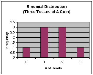
Either by calculating or by looking at the tree diagram, we can ask ourselves:
These probabilities form a binomial distribution.

Calculating probabilities when there are many ways that an
event can happen--and not happen--can be quite difficult, because there
are many factorial expansions (such as N!). So, sometimes
we use an approximation of the Binomial Distribution--which
is the Poisson Distribution. This distribution is
particularly useful for rare events with a large sample size--
that is, when you're trying to predict the (very small) likelihood that
a something unusual will happen.
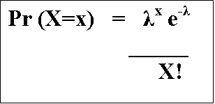
The formula for the Poisson probability is:

Let's go through this step-by-step.
Let's think about that example of finding 15 red cars in a parking lot with 200 cars (given that the expected frequency of red cars is 10%).
So, plugging in the numbers would give us

The 1019 and the 10-9 collapse down to 1010,
which leads us to

The 1010 divided by the 1012 reduces down to 1 / 102,
or 1 / 100, and the 6.754 / 1.3076 = 5.165, which leads us to...

That's a pretty close approximation to what we would get if we used the
binomial distribution formula.
Poisson probabilities are particularly useful in genetics because you might
want to calculate the probabilities for events which are rare compared to a
large potential sample size--i.e., the likelihood of a particular genotype might
be expected to occur only a few times in the population. Given the size of the population,
it would be almost impossible to calculate out the binomial probability--but
the Poisson is often used, because it easier to work with (given all the cancelling out
that we saw above).
Recall our distinction between aleatory probabilities--
which are probabilities based on a known system.
Much more often, we are modeling probabilities based on observation.
Modeling means that we calculate probabilities for a range of outcomes--
based on some summary statistic and our knowledge of some underlying distribution.
So, for instance, suppose we wanted to build a frequency table for "red cars in
parking lots with 200 cars". We could visit a representative parking lot
(that is, take a sample) and calculate out the likelihood that a car was red.
If, in our sample, we found (as above) that 10% of the 200 cars were red,
and we knew that the underlying distribution might be a poisson distribution,
we could then calculate out the poisson distribution.
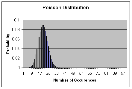
Based on the example above, the distribution (up to 100 red cars) would look
something like this:

Notice that the Poisson probability distribution in the chart is left skewed--which is to say that
once you move into the right-hand three-quarters of the chart, the probabilities
are very, very small. In the case of finding a red car in a parking lot with
200 red cars, the probability of finding 50 or more red cars is almost 0. The poisson
probability formula is appropriate to use in this case.
These are empirical probabilities--much different from when we
were discussing aleatory probabilities, because we had
full information to the degree possible about the
fair coin or die.